Chapter 5: Quantitative Methods Used In Human Resources
PREDICTIVE STATISTICS: Part 2
Multiple Regression Analysis
Linear regression allows you to predict the value of y given x. One variable allows you to reach a conclusion about another because of correlation and an estimate of its size by an equation. Multiple regression represents the same concept using more than one variable x to predict y. This is useful, as often salary level depends on more than one factor.
The figure below depicts multiple regression:
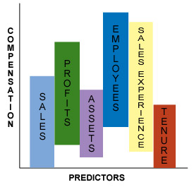
In the figure above, Sales, Profits, Assets, Employees, Sales Experience and Tenure are all x variables or predictors used in a regression formula to predict the y variable, Compensation.
Multiple Regression Model
Multiple regression can be expressed mathematically as:
y = β0 + β1x1 + β2x2 + ... + βkxk + e
In multiple regression, the
- dependent variable y is a function of k independent variables, x1, x2, ... , xk
- value of the coefficient βi determines the contribution of the independent variable xi to the regression line, given that the other x variables are held constant
- β0 is the y-intercept
Using the above illustration, compensation can be written as:
Compensation = β0 + β1 Sales + β2 Profits + β3 Assets + β4 Employees + β5 Sales Experience + β6 Tenure
Each of the coefficients in front of the above independent variables determines how much that independent variable contributes (holding all other variables constant) to the overall regression equation in determining Compensation.
Formulating a multiple regression model
In linear regression, the y and x variables can be visualized in a two-dimensional scatter plot. In multiple regression where multiple x variables are present, the regression line cannot be visualized in two-dimensional space. However, the various coefficients in the above equation can be easily computed using linear regression. For example, you can compute a linear regression equation for Compensation and Sales, Compensation and Profits, etc. The table below shows the coefficients of these independent variables obtained through linear regression:
| Variable | Coefficient |
|---|---|
| Sales | 0.3 |
| Profits | 0.1 |
| Assets | 0.05 |
| Employees | 0.1 |
| Sales Experience | 0.05 |
| Tenure | 0.05 |
Multiple regression combines these linear regression equations in the form:
Compensation = β0 + 0.3 x Sales + 0.1 x Profits + 0.05 x Assets + 0.1 x Employees + 0.05 x Sales Experience + 0.05 x Tenure
The magnitude of the coefficient determines how good of a predictor it is. In the above equation, Sales is the best predictor of Compensation because it has the largest coefficient of 0.3.
Interpreting ANOVA (Analysis of Variance) Outputs
There are several available software products that will model a regression equation for you. (Microsoft's Excel spreadsheet application also has a feature that allows you to run a regression equation.) When these software applications are used, the output often comes in a standard ANOVA format. Click here for a sample ANOVA output that will be used as a reference in this and the next few sections.
There are several components that a regression output will give you. Only a few are essential to your analysis. Those important components are bolded in the sample ANOVA output.
Writing the Regression Equation From the Output
Although the regression output does not give you the overall regression equation, it gives out all the information that you would need to write the regression equation yourself.
Remember the basic form of a multiple regression equation:
y = β0 + β1x1 + β2x2 + ... + βkxk + e
y is the dependent variable, in this case, it is Compensation.
β0 is the y-intercept, in this case, it is equal to 20,951.14.(It is the first line of the third table labeled Intercept from the ANOVA output.)
β1, β2, etc., are coefficients of their respective variable. In this case:
β1 equals 0.0450, which is the coefficient of the Sales variable
β2 equals -0.00034, which is the coefficient of the Profits variable
β3 equals -7.2-5, which is the coefficient of the Assets variable
β4 equals -0.0303, which is the coefficient of the Employees variable
β5 equals -65.8086, which is the coefficient of the Sales Experience variable
β6 equals -22.3804, which is the coefficient of the Tenure variable
The overall regression equation is:
Compensation = 20,951.14 + 0.045 Sales - 0.00034 Profits - 7.2-5 Assets - 0.030 Employees - 65.81 Sales Experience - 22.38 Tenure
Note the random assignment of signs. Also, tenure, profits and assets are known to be good predictors of compensation. However, they all have a negative sign in front of them, indicating that as compensation goes up, these factors go down, which does not make sense. These factors and the large standard error imply that collinearity might exist, such as a linear relationship between two or more variables.
Partial correlation
In multiple regression, because multiple variables are used, often times there is inter-correlation between the variables. This is called collinearity. Collinearity occurs when independent variables are so highly correlated that their individual contribution to the dependent variable is hard to determine. Collinearity does not affect the ability of the regression equation to predict the dependent variable. Collinearity does affect your ability to estimate their individual coefficients. Collinearity exists when the following are present from your ANOVA output:
- Correlation coefficients change dramatically when certain ones are added or removed from the regression model.
- There are large standard errors.
- Independent variables that are highly correlated and therefore are good predictors of the dependent variable may have coefficients that are insignificant.
- Collinear variables may have large coefficients with randomly assigned signs.
If you suspect that collinearity exists, choose your predictors carefully when setting up your regression model. Collinearity is fixed by trial-and-error testing of the different predictors.
R Square
R2 is the same measure that was talked about in the Correlation section. It is also called the coefficient of determination (COD). R Square tells you how successful the predictors were at explaining away the variation in the dependent variable. From the Summary Output, you can see that R Square is approximately 0.21. This means that Sales, Profits, Assets, Employees, Sales Experience and Tenure explained away approximately 21% of the variability in Compensation.
Depending on your objective of the regression equation, different levels of R Square are sufficient to determine effectiveness of your regression model. If the purpose of your regression model is to predict, you would want a higher R Square, in the order of 0.8. If the purpose of your regression model is to examine relationships between the dependent and independent variables, an R Square in the order of 0.2 would be sufficient.
F statistic
The F statistic measures the fitness of the entire regression equation.
The null hypothesis for the F statistic is that the entire regression equation = 0, or put another way, the regression equation is not significant.
In order to test this null hypothesis, you look at the F statistic in the second table from the ANOVA output. In this case, it is 0.7848. You compare this F statistic to a critical F value. The critical F value differs across textbooks. In this course, we will use 8 as the critical F value.
If the F statistic from the regression output is larger than the critical F value of 8, we reject the null hypothesis.
In this case, we cannot reject the null hypothesis because the F statistic is much lower than the critical F value of 8. That means our regression equation is not significant.
t Statistic
The F statistic allows you to determine the fitness of the overall regression model, while the t statistic allows you to determine the fitness of the individual predictors.
Just as with the F test, the t test also has a null hypothesis and a critical t value. The null hypothesis of the t statistic is that the variable equals 0.
Put another way, the variable is insignificant. The critical t value also differs from textbook to textbook. Here, we will set it at 2.5.
If the absolute value of the t statistic is greater than 2.5, then we reject the null hypothesis.
Looking at the Summary Output, no t statistic is higher than 2.5. That means none of the variables are significant in predicting Compensation. That explains the low R Square, as well as the low F statistic.
Standard error and 95% confidence interval
The standard error can also tell you if the variable is significant. Compare the standard error of the variable to its coefficient. If the standard error is large, that means the variable is probably not significant.
Looking at the Summary Output, all of the standard errors of the variables are rather large. In some cases, they are larger than the coefficients themselves. Remember that a 95% confidence interval is +/- 2 standard errors. If the standard errors are large, +/- 2 standard errors will give you a wide range. If the 95% confidence interval contains the number 0, that means you cannot reject the null hypothesis above and that variable is not significant. All of the 95% confidence intervals above contain the number 0, therefore, none of them are significant.
Transformations
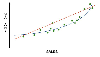
In your regression analysis, sometimes, you will not be able to fit a linear line through the distribution of data points in the graph. For example, consider the following graph:
Data points are clustered in the bottom left corner of the graph. Fitting a line through the above data points would give you the following:
This graph does not allow you to make very good predictions. There are larger variations in y for the smaller x values than for the larger x values. For example, a one-unit increase in x toward the left-hand side of the above graph would give you a large decrease in y. However, a one-unit increase in x toward the right-hand side of the graph would give you a very small decrease in y. In these cases, transformation is used to achieve linearity and constant variance around the regression line.
In transformation, often the y variable is transformed first to achieve constant variance around the regression line, and then the x variable is transformed to achieve linearity. Several types of transformation can be performed, depending on the original structure of the data distribution. Some frequently used transformations are:
- Logs
- x2 or y2
- Square root x or square root y
- 1/x or 1/y
Outliers
Sometimes outliers can also skew a regression line. Outliers are observations that lie far from the main body of the distribution. Histograms can be used to identify outliers. Outliers may result from measurement errors (such as typing errors), or it may be that there are observations that are very different from the rest of the dataset. Outliers must be treated with care. If the outlier is a result of a measurement error, it may be discarded from the dataset. Otherwise, more careful examination of the observation is required. You must first determine the origin of the outlier before you decide whether to include or discard the outlier.
Polynomial Regression
Polynomial regression is a regression technique that fits a predicted equation to a predictive variable in a method that permits a curved line to be the result. While linear regression gives a straight line that always passes through the average of both axes, polynomial regression develops a curved line that passes through these averages.
Polynomial regression equations are best expressed as:
y = β1x + β2x2 + β3x3 + β4x4 + ... + βnxn + b
where y is the variable to be predicted and x is the known variable. (For multiple variables, refer to nonlinear regression below.)
Polynomial regression example
A human resources manager wishes to assign points to a factor in a job evaluation plan such that the points would never be less than 20 and where the values would increase to reflect the job market with bias (racial/sexual) eliminated. In reviewing data for the four factor levels, the following results are shown:
| Level | Predicted Value |
|---|---|
| 1 | 200 |
| 2 | 750 |
| 3 | 2,000 |
| 4 | 4,250 |
| 5 | 7,800 |
If the coefficients are not important, what might the equation look like?
Polynomial regression solution
Examine the values for the various powers.
| x | x2 | x3 | Predicted Value |
|---|---|---|---|
| 1 | 1 | 1 | 200 |
| 2 | 4 | 8 | 750 |
| 3 | 9 | 27 | 2,000 |
| 4 | 16 | 64 | 4,250 |
| 5 | 25 | 125 | 7,800 |
y = β1x + β2x2 + β3x3 + b
y = 50x + 50x2 + 50x3 + 50
Because of the complications in solving for polynomial expressions, and because we know of no instance where this is done entirely by hand, we suggest using statistical or other software to solve the above equation.
Internet Based Benefits & Compensation Administration
Thomas J. Atchison
David W. Belcher
David J. Thomsen
ERI Economic Research Institute
Copyright © 2000 -
Library of Congress Cataloging-in-Publication Data
HF5549.5.C67B45 1987 658.3'2 86-25494 ISBN 0-13-154790-9
Previously published under the title of Wage and Salary Administration.
The framework for this text was originally copyrighted in 1987, 1974, 1962, and 1955 by Prentice-Hall, Inc. All rights were acquired by ERI in 2000 via reverted rights from the Belcher Scholarship Foundation and Thomas Atchison.
All rights reserved. No part of this text may be reproduced for sale, in any form or by any means, without permission in writing from ERI Economic Research Institute. Students may download and print chapters, graphs, and case studies from this text via an Internet browser for their personal use.
Printed in the United States of America
10 9 8 7 6 5 4 3 2 1
ISBN 0-13-154790-9 01


The ERI Distance Learning Center is registered with the National Association of State Boards of Accountancy (NASBA) as a sponsor of continuing professional education on the National Registry of CPE Sponsors. State boards of accountancy have final authority on the acceptance of individual courses for CPE credit. Complaints regarding registered sponsors may be submitted to the National Registry of CPE Sponsors through its website: www.learningmarket.org.