Chapter 5: Quantitative Methods Used In Human Resources
PREDICTIVE STATISTICS: Part 1
Regression Analyses
In compensation administration, information such as the salary or benefits levels offered by other companies are often of interest to human resource professionals. You can select random samples of salaries or benefit levels and use their means to predict the salary or benefits level of interest to you. However, this technique leaves out important factors that affect salary and/or benefits. For instance, experience, performance levels, company size and revenue, etc., play important roles in salary determination.
Regression analyses allow human resources professionals to consider all these factors in setting pay and benefits levels.
- Linear Regression allows you to make predictions of any dependent variable (y) based on any independent variable (x).
- Multiple regression allows you to make predictions of any dependent variable (y) based on several independent variables (x).
Linear Regression
We will first discuss how to conduct linear regression analyses.
Straight-line model
On a graph of the variables, each x value is plotted on the x-axis (horizontal line), and each y value is plotted on the y-axis (vertical line). Each x value and its related y value make up the coordinates of each point. After all the points have been plotted on a graph, the result is known as a scatter diagram.
A scatter diagram helps you to visualize the relationship, if any, between the x and y variables.
When this relationship is linear, as it is above, the 2 variables (x and y) are related; then it is possible to predict values of y from various values of x. This prediction comes from finding the straight line that best fit the data.
Least-squares model
The least-squares method is used to find the straight line that best fits the data. It is based on the principle that a line of best fit, or one that describes a relationship between two variables best, is a line for which the sum of the squares of the deviations or differences between values on the straight line itself and the actual values will be at a minimum. Only one line of the infinite number available may be drawn to meet this requirement. The line of best fit must be computed mathematically, and it will always pass through the average of the x and y data.
The equation for this line is best expressed as:
y = β0 + β1x + Ɛ
| y | dependent variable |
| x | independent variable or predictor (used as a predictor of y) |
| Ɛ | random error or residual (actual y value - mean of y) |
| β0 | y-intercept |
| β1 | slope |
We can use this equation to predict any y value when we know the value of x. A graphical representation of this equation is below:
One can visually approximate the position of a line of least squares through data plots by calculating the means of both axes. Regression lines always pass through these two means on any data plot.
Line of best fit
The line of best fit is the line that produces the best estimate of y based on any given value of x. One way to decide quantitatively how well a line fits the data points is to calculate the extent to which the data points deviate from the line. This deviation or error is the vertical distance between the data point and the line. If you take the deviation or error for each of the data points, square them, then add them together, you have a sum of squared errors (SSE). The line that produces the smallest SSE is the line of best fit.
 denotes the value of y predicted from the visually fitted model.
The best-fit line is the line with the smallest SSE (sum of squares of the errors), which is a measure of the extent to which the data points deviate from the line. Using the graph above, the data can be summarized as:
The sum of errors equals 0, and the sum of squares of the errors (SSE) equals 2. Drawing different lines through the above graph would result in different values for the sum of errors and the SSE, but only the line with the smallest SSE would be the above regression line with an SSE of 2.
How to find the least squares line
To find the least squares line for a set of data, you must find
 and , which are least squares estimates of the population parameters
β0 and β1.
and , which are least squares estimates of the population parameters
β0 and β1.
For a sample of 5 data points in the table above, the fitted line is represented as:
ŷ = ![]() +
+ ![]() x
x
The "hats" are read as "estimator of." In this case, ŷ is the
estimator of the mean value of y.
![]() and
and ![]() are estimators of
β0 and β1.
are estimators of
β0 and β1.
Least-square estimates can be expressed mathematically as:
It should be noted that the higher the correlation (r) between x and y, the better the line will fit the data. The purpose of regression is to extract all possible information from the data. The regression model should explain as much as possible about the underlying process. However, due to real world uncertainty, no model will explain everything. The information in the data that are not explained by the regression model is the error component called residuals.
Example of linear regression
The following data is a summary of of a salary structure. Calculate the regression equation.
| Sample | Grade | Weekly Salary ($)* |
|---|---|---|
| A | 4 | 1000 |
| B | 6 | 2000 |
| C | 6 | 3000 |
| D | 10 | 3000 |
| E | 10 | 4000 |
| F | 12 | 5000 |
In the summary below, the data in the grade column is used for the x variables. The data in the weekly salary column is used for y, but it is divided by 1000 to simplify the calculations.
The data from above can be summarized in the table below:
The equation for linear regression is:
β1 = 0.4167
The regression line passes through the averages of the data, therefore, β0 equals:
y = β0 + (0.4167)(x)
3 = β0 + (0.4167)(8)
3 = β0 + 3.334
β0 = −0.334
This gives us an equation for a line in the form y = mx + b.
y = (0.4167)x + (-0.334)
Implication: If you know x, which in this case is the performance level, you can use the above regression model to find the appropriate salary based on the given salary structure.
Correlation and Predictive Reliability
Sometimes it is useful to set pay based upon measurable factors such as past performance level or education. In this case, correlation may be used to determine what the relationship is between these factors and pay level.
Correlation is a measure of the association of values of x and y. That is to say, correlation does not measure "causality," but it does show the extent to which you are likely to find a given value of y (say a) when you know the value of x (say b). If you find a, you are likely to find b; that does not mean that a causes b.
For instance, statistically, there is a high degree of correlation between CEO performance and company revenue. However, there is no indication that one causes the other.
Correlation coefficient is a measure of the dispersion of data points around a straight line. It is exhibited on a scale of -1 to 1.
- 1 = positive correlation
- -1 = negative correlation
- 0 = no correlation
| Correlation Coefficient | Behavior |
|---|---|
| 0 | No correlation between x and y. |
| 1 | As x increases by 1, y increases by exactly 1. |
| -1 | As x increases by 1, y decreases by exactly 1. |
| negative | x and y move in opposing directions. As x increases, y decreases. |
| positive | x and y move in the same direction in a like manner. As x increases, so does y. |
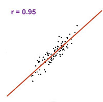
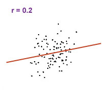
The size of the correlation coefficient indicates the strength of the relationship between x and y. The closer the coefficient is to 1 (either + or -), the more likely you'll find y given x. Below are some sample correlation graphs of various correlation coefficients:
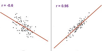
Note that with a higher coefficient (0.95), the dispersion of data points are tighter around the line compared to a lower coefficient of -0.6.
The correlation coefficient (r) can be expressed in the following mathematical form:
| xi, yi | x and y observations |
| x | the mean of x |
| y | the mean of y |
| SD (x) | standard deviation of x |
| SD (y) | standard deviation of y |
Correlation and Predictive Reliability
Correlation is a measurement of direction and relationship between 2 variables. But correlation is not as useful a measurement as its square, r2, the Coefficient of Determination (COD). Typically used in regression analyses, r2 represents the fraction of variability in y that can be explained by the variability in x. In other words, r2 explains how much of the variability in the y can be explained by the fact that they are related to x, i.e., how close the points are to the regression line.
The coefficient of determination indicates how much of the total variation in the dependent variable can be accounted for by the regression function. For example, a COD of 0.7 implies that 70% of the variation in y is accounted for by regressing it on x.
The COD (r2) can be expressed mathematically as:
| yi | y observations |
| y | the mean of y |
| ŷ | residual |
ŷ equals the residual or what's left over after the regression has explained away all the variability of the dependent variable.
Example of coefficient of determination
Consider the following 2cases:
- Executive compensation vs. company revenue
- Factory worker vs. company revenue
The correlation coefficient (r) of:
- executive compensation vs. evenue is 0.95
- factory worker compensation vs. company revenue is 0.2
To find the COD, square the correlation coefficients.
(0.95)2 = 0.9025
(0.2)2 = 0.04
This results in an r2 of 0.9025 for executive compensation vs. company revenue, compared to an r2 of 0.04 for factory worker compensation vs. company revenue.
 |
 |
Executive compensation vs. company revenue |
Factory worker compensation vs. company revenue |
Interpretation: 90% of the variation in executive compensation can be attributed to differences in company revenues, while only 4% of the variation in factory worker compensation can be attributed to differences in company revenues. This means company revenue is NOT a good predictor of factory workers' compensation.
Standard Error
The standard error is an estimate of the variability or random error of the sample to the population.
Example: A population has a mean of 6. You would expect that samples taken from this population would also have means of 6. However, that is rarely the case. The means of the samples taken from this population will vary due to sampling errors. Standard error is a measure of any differences that the sample has from the true mean of the population.
Standard error is defined as:

| S | standard error |
| s | standard deviation |
| n | sample size |
Consider the dataset below. Drawing different samples from the dataset would give you different means and different standard deviations.
| Employee | Base Salary ($)* |
|---|---|
| A | 85,397 |
| B | 108,396 |
| C | 119,037 |
| D | 120,064 |
| E | 190,972 |
| F | 103,873 |
| G | 93,835 |
| H | 97,734 |
Different samples lead to different statistics.
When relying on salary survey data to set pay, you must ask:
- Does this survey report a standard error?
- If so, how large is the standard error?
The standard error answers the question: "Is this sample very different from all the other possible samples that could be drawn from this population?"
In general...
The smaller the population and the more biased the sampling method, the larger the error will be.
Example of standard error
What is the standard error of a sample of 10 observations with the standard deviation of 28,892?
Internet Based Benefits & Compensation Administration
Thomas J. Atchison
David W. Belcher
David J. Thomsen
ERI Economic Research Institute
Copyright © 2000 -
Library of Congress Cataloging-in-Publication Data
HF5549.5.C67B45 1987 658.3'2 86-25494 ISBN 0-13-154790-9
Previously published under the title of Wage and Salary Administration.
The framework for this text was originally copyrighted in 1987, 1974, 1962, and 1955 by Prentice-Hall, Inc. All rights were acquired by ERI in 2000 via reverted rights from the Belcher Scholarship Foundation and Thomas Atchison.
All rights reserved. No part of this text may be reproduced for sale, in any form or by any means, without permission in writing from ERI Economic Research Institute. Students may download and print chapters, graphs, and case studies from this text via an Internet browser for their personal use.
Printed in the United States of America
10 9 8 7 6 5 4 3 2 1
ISBN 0-13-154790-9 01


The ERI Distance Learning Center is registered with the National Association of State Boards of Accountancy (NASBA) as a sponsor of continuing professional education on the National Registry of CPE Sponsors. State boards of accountancy have final authority on the acceptance of individual courses for CPE credit. Complaints regarding registered sponsors may be submitted to the National Registry of CPE Sponsors through its website: www.learningmarket.org.