Chapter 5: Quantitative Methods Used In Human Resources
STATISTICAL TERMINOLOGY
Statistical Symbols
This insert shows commonly used symbols that designate a variety of statistical terms. In some instances, a term may be denoted by more than one symbol. In general, population statistics are denoted by Greek letters and sample statistics are denoted by Roman letters.
| Symbol | Term or Concept |
|---|---|
| X (read: X bar) | mean of sample |
| μ (read: mew) | mean of population |
| | | | absolute value: ignore + or - sign |
| = | equal or equivalent to |
| s | standard deviation of sample |
| σ (read: sigma) | standard deviation of population |
| Σ (read: Sigma) | summation |
| > | greater than |
| < | less than |
| ≥ | equal to or greater than |
| ≤ | equal to or less than |
| log | logarithm to base 10 |
| In | logarithm to base e |
| n | number of cases in a sample |
| N | number of cases in a population |
| f | frequency |
| Q | quartile |
| D | decile |
| R | range |
| r | correlation |
| r2 | explained variance or coefficient of determination |
| X | an independent variable |
| Y | a dependent variable |
| Xi | one of several independent variables |
| A ( or b0) | constant in a regression equation from sample data |
| B (or bi ) | coefficient of X (or Xi) in a regression from sample data |
Population
In salary surveys or analyses, the universe of observations of interest to a human resources manager is generally called a population. The characteristic that defines the population is called the parameter. In a salary survey, we might be interested in a population of all jobs in all companies in an industry. The parameter with which we would be concerned might be salary.
Any summary measure of a population is called a parametric value.For instance, the average salary for all clerks in the industry: "clerks' average salary" is a parametric value.
Since administrators are concerned with the general applicability of their findings, they are concerned with statements they can make about a total population. (For example, only four of ten companies may have agreed to participate in a survey -- which would have a great deal of impact on the applicability of the results to the entire population.)
Making valid inferences about populations is the highest order of generalization possible. In some cases, however, a population cannot be examined in its entirety: it may be infinite; it may be such a large finite population that it is impractical to handle all possible observations; or you may not receive the necessary cooperation. The researcher then must take a "shortcut" consisting of approximating the population by studying a sample of observations from that population.
Population example
You wish to conduct a survey of management positions in the glass industry. What would constitute a "sample" of the population?
Population solution
Survey definition:
Population: Names (and N) of all companies in the industry
Sample: Names (and N) of all companies participating in the survey
Samples
Sampling consists of obtaining observations on a restricted number of events that comprise the entire population. A sample is a finite portion of the population. There are a number of ways in which samples may be obtained.
The most common form is random sampling. Random sampling is the process that assures no single observation is selected for inclusion in the sample in such a way that it is favored over any other observation. Each observation in the population has an equal chance of being included in the sample. When one or another observation is favored for inclusion in the sample, the sample is no longer considered random and is not representative of the population; it is then said to be "biased."
Sampling constitutes the essence of survey methodology; hence, it will be covered more fully in later discussions.
Sample example
A major national survey sends you these results for Los Angeles:
| Secretaries | Number of Companies | Number of Positions | Median | Mean |
|---|---|---|---|---|
| Junior | 5 | 17 | $35,600 | $37,000 |
| Senior | 18 | 56 | $41,000 | $42,000 |
| Executive | 12 | 13 | $66,000 | $68,000 |
Comment on the results as defined by the information above.
Sample solution
The sample is very small (Los Angeles has over 2,000 companies with more than 100 employees.)
- The sample may be biased.
- The sample may not be random.
- Medians are lower than averages.
One may hesitate to use these results.
Range
A range (R) is a summary of numerical observations. It is an index of the extent of the spread of the observations between the empirically determined limits low (l) and high (h). The range is determined by subtracting the value of the lowest reported observation from the value of the highest.
For example, for reported income levels with the lowest observation of $11,000 and the highest at $35,000:
R = Xh- X
R = $35,000 - $11,000
R = $24,000
The interquartile range (Q) is most often used as a measure of distribution. Q is equal to the range of the middle 50% of the observations in a distribution also referred to as the interquartile range as mentioned earlier. It is equal to the range of the observations that lie between the 25th and 75th percentile, or as previously defined: Q1 (25th Percentile) and Q3 (75th Percentile).
Range example
From the following data, what is the sample's range, and what is the interquartile range? How would you select a salary range for a structure?
Sample Position Salaries:
| $20,000 | $30,000 | $34,000 |
| $24,000 | $30,000 | $36,000 |
| $24,000 | $30,000 | $38,000 |
| $26,000 | $30,000 | $40,000 |
| $28,000 | $34,000 | $64,000 |
Range solution
The range is $20,000 to $64,000.
The interquartile range is $26,000 to $36,000.
Salary ranges for structures are usually arbitrarily set. Percentage differences may vary from 20%-50% at the bottom to 40%-70% at the top. A few companies utilize the interquartile range, but they are rare.
Distributions
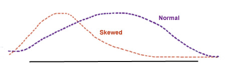
Normal: Normal distributions are defined as a "bell shaped curve." They represent a standard distribution and are a model around which many statistical tests have been devised. When a distribution from the real world matches a normal distribution, these tests can then be transferred to describe the "real world model."
Skewed: Often the top of the curve will be displaced to the right or left. This is known as a "skewed distribution." Annual salaries, for instance, are reported by government agencies in terms of median income. The median income reflects more closely the typical income than the mean income would. This is because most wage earners tend to receive salaries that are at the lower end of the scale of all possible salaries. Thus, mean income would place an undue weight on salaries that are far up on the scale -- of which there are relatively few.
This is defined in statistics as the "skewness" of the distribution. The preceding example gives evidence of this.
Distribution example
Would you expect management salaries, as well as clerical salaries, to have a skewed distribution?
Distribution solution
Yes. For example, the following graph might represent controllers' salaries for $100 million companies.
Frequency Distributions
One of the most important differences between samples and populations of observations is the differential distribution of observed values among the possible categories. Looking at any data, the nature of this distribution can be determined by determining the frequency of each observation's occurrence.
One convenient method for doing this is to set up a "tally sheet." The tally sheet is a summary sheet consisting of all possible categories within a range of observed values, as in the example:
| Salary | Men | Women |
|---|---|---|
| $15,000 - $20,000 | 8 | 57 |
| $20,000 - $35,000 | 28 | 17 |
| $35,000 - $40,000 | 42 | 6 |
In this sheet, the salary categories are:
- $15,000 to $20,000
- $20,000 to $35,000
- $35,000 to $40,000
The tally summarizes the occurrence of events (how many men and how many women receive a specified salary in each category).
Frequency example
Draw a frequency distribution for the following data using increments of three for classification:
| 1 | 6 |
| 1 | 7 |
| 2 | 8 |
| 3 | 10 |
| 4 | 11 |
| 5 | 12 |
| 6 |
Frequency solution
Frequency distributions for the data given in categories by increments of three are:
| Frequency Classes | Counts |
|---|---|
| 1 - 3 | 4 |
| 4 - 6 | 4 |
| 7 - 9 | 2 |
| 10 - 12 | 3 |
Variance and Standard Deviation
The Variance (S2) of a distribution is the mean of the squared deviations of the observations in a distribution subtracted from the mean of the distributions.
The standard deviation (S, or you may see Sd being used, too) is the amount by which all observations differ from the norm, and it is the square root of the variance.
where:
X = the sample
X = Average (mean) of the sample
n = number of observations in the sample
Both these terms (standard deviation and variance) refer to the same amount by which a sample varies.
For example, if X is the sample, and X is the mean:
| X | X | X - X | (X - X)2 |
|---|---|---|---|
| 30 | 31 | -1 | 1 |
| 16 | 31 | -15 | 225 |
| 40 | 31 | 9 | 81 |
| 36 | 31 | 5 | 25 |
| 39 | 31 | 8 | 64 |
| 34 | 31 | 3 | 9 |
| 37 | 31 | 6 | 36 |
| 10 | 31 | -21 | 441 |
| 18 | 31 | -13 | 169 |
| 50 | 31 | 19 | 361 |
| 310 | 0 | 1,412 |

These numbers provide a method by which one can estimate the distribution for a sample. For any sample, one can expect that roughly two-thirds of the sample will fall within one standard deviation plus or minus the mean. In our example, this would put the distribution of that two-thirds from 19 to 43.
Variance and standard deviation example
- Can a variance or a standard deviation be computed as a negative number?
- Compute a standard deviation from the following performance summary ratings:
1 3 5 2 2 2 4 5
Variance and standard deviation solution
- Since the variance of a distribution is the mean of the squared deviations of the observations, variances will always be a positive number. Because the variance is always a positive number, the standard deviation (which is the square root of the variance) will be also be a positive number.
-
X X X - X (X - X)2 1 3 -2 4 3 3 0 0 5 3 2 4 2 3 -1 1 2 3 -1 1 2 3 -1 1 4 3 1 1 5 3 2 4 24 0 16
X = SX / n
X = 24 / 8
X = 3


For larger populations, use:
Correlation
Correlation techniques aid administrators in predicting the value of one variable when given the value of another variable. Correlation itself is a measure of the association of values of x and y populations. That is to say, correlation does not measure "causality," but it does show the extent to which one is likely to find a given value of y (say a) when one knows the value of x (say b). If you find a, you are likely to find b; that does not mean that a causes b.
For instance, statistically, there is a high degree of correlation between the number of births in Des Moines, Iowa and the rainfall in Bombay. There is no indication that one causes the other.
Correlation is exhibited on a scale of -1 to 1.
A correlation of 0 means that there is no correlation between x and y. A positive correlation means that x and y move in the same direction in a like manner. A negative correlation means that x and y move in different directions.
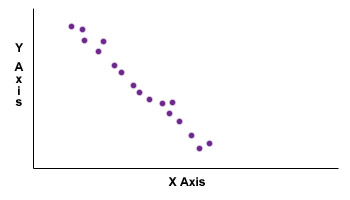
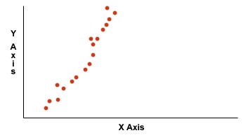
Example of a positive correlation
Regression: Closely related to correlation is regression analysis. This is a procedure used to make predictions based on correlated data. For instance, given two variables (such as height and weight) one may predict the average of one (e.g., height) when given the value for the other (i.e., weight).
Regression analysis is also known as:
- line of best fit
- line of averages
- line of least squares
Regression is a frequently utilized tool for analytical procedures in human resources.
Regression example
Can you describe the arithmetic formula for the line shown above?
Regression solution
The formula for linear regression (determination of the line of best fit) is:
y = mx + b
| y | the dependent variable |
| x | the independent variable |
| b | the constant of "intercept" where the line crosses the y-axis and x = 0 |
| m | the slope of the line |
Internet Based Benefits & Compensation Administration
Thomas J. Atchison
David W. Belcher
David J. Thomsen
ERI Economic Research Institute
Copyright © 2000 -
Library of Congress Cataloging-in-Publication Data
HF5549.5.C67B45 1987 658.3'2 86-25494 ISBN 0-13-154790-9
Previously published under the title of Wage and Salary Administration.
The framework for this text was originally copyrighted in 1987, 1974, 1962, and 1955 by Prentice-Hall, Inc. All rights were acquired by ERI in 2000 via reverted rights from the Belcher Scholarship Foundation and Thomas Atchison.
All rights reserved. No part of this text may be reproduced for sale, in any form or by any means, without permission in writing from ERI Economic Research Institute. Students may download and print chapters, graphs, and case studies from this text via an Internet browser for their personal use.
Printed in the United States of America
10 9 8 7 6 5 4 3 2 1
ISBN 0-13-154790-9 01


The ERI Distance Learning Center is registered with the National Association of State Boards of Accountancy (NASBA) as a sponsor of continuing professional education on the National Registry of CPE Sponsors. State boards of accountancy have final authority on the acceptance of individual courses for CPE credit. Complaints regarding registered sponsors may be submitted to the National Registry of CPE Sponsors through its website: www.learningmarket.org.