Chapter 5: Quantitative Methods Used In Human Resources

Overview: An overview of the basic quantitative methods human resource professionals rely upon to administer compensation and benefits programs.

Corresponding courses

09 Basic Quantitative Methods

19 Quantitative Methods Used in Salary Administration

49 Regression Analyses Used in Compensation Administration

MATHEMATICAL SYSTEMS

Human resource practitioners intuitively use a mathematical system when they apply quantitative methods to solve business problems. A mathematical system depends on:

1. A set of elements (such as rational numbers, whole numbers, etc.)
2. Operations that can be applied to the set of elements (such as addition, multiplication, etc.)
3. One or more relationships (such as the equation: 1 + 1 = 2)
4. Axioms that are accepted rules (e.g., the rule of identity which is expressed in the equation a = a)

While any system can be used, human resource practitioners are accustomed to the simple rules and operations of the arithmetic system of real numbers. Statistical practices often require the application of special rules and operations within the set of rules of the mathematical system. In a sense, that makes the statistical methods, a "subset" of the entire mathematical system that we use. This is essential to remember since statistical methods cannot exceed the limitations of normal mathematical boundaries. It is also important to remember that not all the tests or approaches may be appropriate, because the boundaries of normal mathematics might be exceeded in given situations.

In statistics, these boundaries are called assumptions.¹

Mathematical Systems Example

What are the assumptions that a normal statistical review (e.g., bell-shaped curve) might require in comparing the results of performance appraisals between men and women in your organization?

Mathematical Systems Solution

1. The observations must be independent. That is, one measurement should not bias the other.
2. The measurements must be from a normally distributed population. That is, the traditional "bell-shaped" curve.
3. The populations must have the same variance (explained later).
4. The measurement must be of at least an interval scale (also to be explained).
5. The effects must be additive.

Without more detailed information, the example of performance appraisal measurement exceeds all these boundaries.²

TYPES OF MEASUREMENTS

There are four basic kinds of measurements:

1. Nominal
2. Ordinal
3. Interval
4. Ratio

Nominal Measurements

The first of these, nominal measurements (or scales) are composed of numerical values that serve to identify discrete categories; i.e., the numbers are labels for the categories and imply no quantitative (measurable) differences that can be handled meaningfully in numerical operations. The numbers on front doors, for instance, constitute such a scale; Social Security numbers are another example.

In salary surveys, the numbering of positions or companies is just such a scale; the numbers are used merely as labels.

* The numbers are used for illustration purposes only.

Company Name	Company Number	Position	Position Number	Salary*
ABC Company	021	Secretary	91	$24,000
ABC Company	021	Clerk	92	$22,000
ABC Company	021	Typist	93	$16,000
XYZ Company	043	CEO	11	$166,000
XYZ Company	043	Clerk	92	$18,000

Nominal measurements example

You are about to conduct a survey of five positions, and you have numbered them as follows:

Position	Position Number
Secretary	1
Stenographer	4
Clerk	2
Typist	5
CEO	3

What significant computations can be completed using the position numbers?

Nominal measurements solution

No SIGNIFICANT computations can be completed.

For example: 1 + 2 + 3 + 4 + 5 = 15 means nothing.

Nominal measurements allow only the most limited application. For example, one can count classes (the numbers of positions numbered "2" for instance). Or "Yes" - "No" can be counted where 0 - 1 correspond to "yes" and "no." However, most human resource administrators will find that using nominal measurements in any kind of mathematical operation is bound to lead to error. For instance:

Employee's Social Security Number:	536-41-3760
	+
Spouse's Social Security Number:	437-28-5621
TOTAL:	973-69-9381

is a totally meaningless number.

Ordinal Measurements

Ordinal measurements have, in addition to nominal properties, rank differences. That is, the numerical value of these scales indicates that there are not only differences between categories but that these are quantifiable differences. An ordinal scale ranks "observations" with regard to the extent to which they possess more or less of a given quality. The ranks do not, however, indicate the degree of difference (how much more or less) of the property each observation has.

There are events with dimensions that cannot be readily quantified. It would be absurd to state that a painting is twice as beautiful as another or that one restaurant has food one-third as tasty as another. For this reason, ordinal scales are often applied to observed events that differ along qualitative rather than quantitative dimensions (especially when the qualitative dimension cannot be easily expressed quantitatively).

For example, in job evaluation plans, the following factors cannot be easily broken down into quantifiable units:

• problem complexity
• responsibility
• human/social challenges
• skill
• authority
• impact on profit

Can one job have two times as much the problem complexity as another? However, within each factor there can be a breakdown of steps.

For example, problem complexity might be broken down by:

Rank Number	Rank
1	Repetitive
2	Moderately Complex
3	Very Complex
4	Extremely Complex

These steps may be described as "ordinally ranked."

Ordinal measurements example

You have been asked to estimate the average salaries of individuals within the United States who hold the following degrees:

• PhD
• MBA
• BS
• BA
• High School Diploma

Ordinal measurements solution

Average salaries by degree:

*The numbers are used for illustration purposes only.

Degree	Salary*
PhD	$61,891
MBA	$82,463
BS	$50,438
BA	$47,625
High School Diploma	$31,112

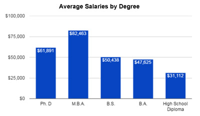
This measurement is very important. Performance appraisals are almost always on ordinal scales, yet human resource practitioners often try to utilize mathematical tests and computations that require more stringent assumptions.

Interval Measurements

Interval scales are equal unit scales; that is, the distance between adjacent units on an interval scale is the same, irrespective of the magnitude of the adjacent scale units. For instance, the distance between $5,000 and $6,000 is the same as the distance between $61,000 and $62,000, since it reflects a measurable increase in real dollars.

Interval scales, however, are only relative. For example, if these amounts ($5,000 - $6,000 and $61,000 - $62,000) were to represent sales compensation, the amount of actual sales required to produce the increase in sales compensation in the above example may be different at $5,000 (to $6,000) and $61,000 (to $62,000). Thus, the dollar scale may reflect relative rather than absolute changes. For example:

Sales ($)	Broker's Commission ($)	Salesman's Commission ($)
20,000	0	0
40,000	500	300
60,000	1,500	900
120,000	4,500	2,700

Interval scales are the most frequently used measurement in human resource pay practices. However, many human resource measurements cannot satisfy the requirements that measurements be similar and equidistant in their measurement intervals. Their ordinal or nominal characteristics must be recognized in order to understand the explanations of tests discussed later in this chapter.

Interval measurements example

A salesman sells a product for $90,000. His broker's commission is 5% after the first $30,000. The salesman receives 60% of this broker's commission. What is the salesman's commission?

Interval measurements solution

Salesperson's commission:

Revenue - Base = Commissionable Revenue
$90,000 - $30,000 = $60,000

Commissionable Revenue x Broker's Percentage = Total Commission
$60,000 x 0.05 = $3,000

Total Commission x Salesman's Percentage = Salesman's Commission
$3,000 x 0.60 = $1,800

Special note: These plans are often increased or decreased in specific percentage amounts for:

1. special product mix
2. new client solicitation
3. new market or product introduction
4. administrative effectiveness
5. other variables

Salesmen operate (and are motivated) on ordinal rates via interval increases.

Ratio Measurements

The ratio scale has, in addition to the properties of the nominal, ordinal and interval scales, an absolute zero. The absolute zero represents a point below which no value can be assigned. Zero represents no less than one of the property being gauged by the scale. In salary administration, for example, dollars in value can be shown on the interval scale, while percentages can be shown on a ratio scale. Compensation dollars, however, can be ratio ( i.e., if no negative exists).

(One must remember that division by zero is not an acceptable mathematical operation. Hence, ratio measurements have certain computational limitations.)

Examples of ratio measurements include:

Sales ($) $0 Base	Expenses ($) $0 Base	ExpenseRatio $0 Base
1,000,000	Rent = 5,000	0.5%
	Travel = 50,000	5.0%
	Salaries = 500,000	50.0%
	Benefits = 175,000	17.5%

Ratio measurements example

You have three departments, each of which has budgeted the following salary increases for the coming year:

Department A: 7% raise for 2 employees
Department B: 9% raise for 3 employees
Department C: 11% raise for 95 employees

All employees are receiving $10,000 annual base salaries.

What is the overall budgeted salary increase for the coming year?

Ratio measurements solution

All individuals receive $10,000/year salaries.

Dept.	Number of Employees	% Increase	Total Base Salary ($)	Total Salary Increase ($)
A	2	7	20,000	1,400
B	3	9	30,000	2,700
C	95	11	950,000	104,500
TOTAL	100	27	1,000,000	108,600

Overall increase of salary budget = $108,600 / (100 x $10,000)

Overall increase of salary budget = 10.86%

NOT

Overall increase of salary budget = 27 + 3

Overall increase of salary budget = 9%

This example is designed to illustrate a common error in human resource administration: addition and division of ratios. "Averaging averages" rarely works. As shown above, 9% is not the overall percentage of salary increase because of the equal weight given to departments rather than individuals.

The real average is determined by adding the values of the variables (increases) for all 100 observed events and then dividing that correctly by the number of observations (the total base employees' salaries).

FOUR BASIC MATHEMATICAL OPERATIONS

The basic "statements" of operations in mathematics are statements of equality or inequality. The operation performed on a number or group of numbers is designed to reduce the value to a single number (essentially, to simplify).

The four most common mathematical operations are:

Addition	The process that combines several numbers to obtain a single number whose value equals the total value of the numbers. This operation is usually indicated by the "+" sign.
Substraction	The inverse (the process that reverses an original process) of addition: this operation is the reduction of a number's value by the value of another number (or several numbers in sequence). This operation is usually indicated by a " - " sign.
Multiplication	The process that adds a number to itself a designated number of times; that is, 3 x 4 is merely four 3s added together or 3 + 3 + 3 + 3. This operation is indicated by an "x" sign, the centered period, " ." sign, or an asterisk "*" sign. It may also be understood when a symbol is juxtaposed to a number or another symbol (as in the operation fy, where the value is f x y. Multiplication is also shown if the symbol is next to an operation within parentheses, as in F(3 x 5) where the value is 3 times 5 times F. One always performs operations within parentheses first.
Division	This operation is the inverse of multiplication; that is, the value of the number is reduced into equal parts by a designated number. This operation is indicated by a "÷" sign or by the slanted or horizontal line in a ratio or fraction, as indicated by "/" in the fraction 3/4.

Remember: The operations of multiplication and division are performed first in most statistical packages, unless parentheses indicate a sub-operation to be performed first.

Four basic mathematical operations example

1. Add: 3/7 + 2/9
2. Subtract: 3/7 - 2/9
3. Multiply: 3/7 x 2/9
4. Divide: 3/7 ÷ 2/9

Four basic mathematical operations solution

ADDITION: the process that combines values

a/b + c/d	=	ad + cb bd
3/7 + 2/9	=	(3 x 9) + (2 x 7) (7 x 9)
	=	27 + 14 63
	=	41 63

SUBTRACTION: the process that reduces values

a/b - c/d	=	ad - cb bd
3/7 - 2/9	=	(3 x 9) - (2 x 7) (7 x 9)
	=	27 - 14 63
	=	13 63

MULTIPLICATION: the process that increases the given number

a/b x c/d	=	a x c b x d
3/7 x 2/9	=	3 x 2 7 x 9
	=	6 63
	=	2 21

DIVISION: the process that reduces the value equally

a/b ÷ c/d	=	a/b x d/c
	=	a x d b x c
3/7 ÷ 2/9	=	3 x 9 7 x 2
	=	27 14

Addition

The simplest mathematical computation is addition. Addition combines numbers to make a total called the sum. Of all computations, however, addition, together with its inverse, subtraction, is the source of most computation errors. For years, the IRS has listed addition and subtraction mistakes as the leading cause of faulty returns.

For 2002 and beyond, companies must adopt a vesting schedule at least as generous as those below for employee 401(k) plans:

1. 3-year cliff vesting: 0% vesting for less than 3 years of service; 100% vesting after 3 years
2. 6-year graded vesting: vesting begins in the employees second year of service; it increases by 20% each year, until the employee is fully vested at the beginning of the sixth year of employment

Six-year graded vesting proceeds like this:

Years of Service	Unforfeitable Percentage
2	20
3	40
4	60
5	80
6	100

Addition example

You are 40 years old and have worked for 5 years for your firm. As a participant in the firm's qualified pension plan, what might your non-forfeitable vested pension percentage be in each of the above plans?

Addition solution

Under the 2 different systems, you would be vested as follows:

3-year cliff vesting	100%
6-year graded vesting	80%

Subtraction

Subtraction is the inverse of addition. It calls for the difference in the values of numbers.

Integration with Social Security benefits is a perfect example of how human resource administrators utilize subtraction:

Individual retirement benefit from a retirement plan	$600/month
Amount to be received from Social Security	$400/month
Employer's contribution percentage	37.5%
Employer's portion of $400 Social Security payment	$150/month
FINAL RETIREMENT BENEFIT FROM PLAN	$450/month

Another example would be long-term disability integration and net vs. gross pay computations.

Subtraction example

An employee who would receive a final pension of 50% of last year's earnings in New York decides to retire at age 60 rather than at age 62 (when he would be eligible for the full 50% benefit). What might his percentage be? Remember that an actuarial reduction for early retirement in a defined benefit plan is roughly 5% per year of the benefit (e.g., 3% of a 60% defined benefit).

Subtraction solution

ACTUARIAL REDUCTION
5% of benefit per year = 50% x 5% = 2.5%
(i.e., .50 x .05 = .025 or 2.5%)
50% - 2.5% per year = 50% - (2.5 x 2)
= 50% - 5%
FINAL PENSION = 45%

Municipalities are often not part of the Social Security System, so integration does not apply. In some places, for example, retirement pay is based on a percentage of "last year's earnings"; this includes overtime, hence, occasions have arisen when retirement pay is almost at full last year's base pay.

Multiplication

Multiplication is the computation process that simplifies addition. Factors are combined to give a product.

COMPOUND INTEREST
The compounding of interest refers to the common savings account approach that permits the following increases:

Year 1:	Interest is earned on the sum deposited. (e.g., at 4%, $10,000 would earn $400 in the first year.)
Year 2:	Interest is earned on the original sum deposited (i.e., $10,000) and on the previous year's interest (i.e., $400 more) if the interest is left in the same account. At 4%, $10,000 would still earn $400 in the second year, but now the $400 from the previous year's interest would also be earning 4% interest to make a total of $416 earned in the second year. This makes a total of $10,816.
Year 3:	This process continues indefinitely provided the accumulated interest is left in the same account. For example, the amount in the example above would begin the third year with $10,816 earning 4% on the entire amount.

The formula reads:

Ending Sum = Initial Sum x (1 + Interest Rate)^Years

e.g., $ 10,816 = $ 10,000 x (1 + .04)² *

*It should be remembered that the exponent (power) means that the operation or number should be multiplied by itself that many times. In the example, therefore, the process is (1.0 + . 04)(1.0 +.04). Always perform the operation in parentheses first.

Multiplication example

It is the Year 2020 and the average BA starting salary is $30,000. You predict these starting salaries will increase at a rate of 9% per year. Using the compound interest approach and a calculator, determine a starting salary for a BA in the year 2036.

Multiplication solution

COMPOUND INTEREST

Year	Principal ($)	Interest at 9% ($)
2020	30,000	2,700
2021	32,700	2,943
2022	35,643	3,208
2023	38,851	3,497
2024	42,348	3,811
2025	45,159	4,154
2026	50,313	4,528
2027	54,841	4,936
2028	59,777	5,380
2029	65,167	5,864
2030	71,021	6,392
2031	77,413	6,967
2032	84,380	7,594
2033	91,974	8,278
2034	100,252	9,023
2035	109,275	9,835
2036	119,110

Sum	= Initial Amount x (1 + Interest Rate)Years = $30,000 x (1 + 0.09)(2020 - 2036) = $30,000 x (1.09)16 = $30,000 x 3.970305 = $119,110

Division

Division is the inverse of multiplication. It has the same relationship to multiplication that subtraction has to addition. An inverse cancels the process of its inverse. For example, if you begin with 3 and multiply it by 5 (3 x 5), you need only divide the result (15) by 5 to once again have three. In other words it reversed the original process.

In a division problem such as 15 ÷ 5 = 3, 15 is the dividend, 5 is called the divisor, and the result (3) is the quotient.

Rule of 72

A very useful thing to remember in human resource operations is called "The Rule of 72." If you divide any interest rate into the number 72, your answer will be the number of years it will take for a compound interest rate to double the original sum.

Division example

It is the year 2020 and the average MBA starting salary is $90,000. You predict starting salaries to increase at a rate of 9% per year. Using the Rule of 72, what year will a starting salary for an MBA double to be $180,000?

Division solution

Divide the percentage into 72.

Answer = the number of years required to double the principal.

72 ÷ 9 = 8

2020: $90,000
2028: $180,000

7.2% doubles money in ten years
72 ÷ 7.2 = 10

12% doubles money in six years
72 ÷ 12 = 6

If the inflation rate in 2020 is 12%, how much will a $2.00 loaf of bread cost in the future?

$4.00	in	2026
$8.00	in	2032
$16.00	in	2038
$32.00	in	2044
$64	in	2050

The following sections will show you how to use these mathematical operations for human resource planning, including to determine:

• present value
• logarithms
• averages

Present Value

Salary surveys deal with money, and money accrues a certain value over time. In the traditional sense, money can always be earning interest. The value of $1,000 today is not necessarily what the value of $1,000 might be next year if that sum can earn 10%.

Many human resource decisions involve deferred payments. The collection of their values in a survey would be misleading if they were reported only at their face values.

The computation of the value of the present worth of any sum to be paid in "n" years can be computed thus:

Present value example

A retirement plan promises to pay an individual $10,000 in ten years. If present rates of interest are 10%, what will that $10,000 be truly worth to the individual today?

Present value solution

Present value of compensation dollars depends also on effective tax rates. It is important to remember that in the U.S., maximum tax rates were over 90% 50 years ago. Computations must all estimate this effect -- a difficult task at best.

Logarithms

A logarithm is the exponent of the power to which a fixed number must be raised to produce a given value. For example, if the fixed number is 10 (the most common base), the logarithm of 1,000 is 3. You have to multiply 10 times itself three times (10 x 10 x 10) to produce the desired result (1,000). The logarithm of 10,000 is four.

Logarithms are commonly used in human resource surveys, especially in graphs that show salaries versus some size dimension. The reason for their use is that they allow visual comparison of data that may be quite dissimilar in size.

For example:

SALES ($)	CHARACTERISTIC	+	MANTISSA	=	LOG
25,800,000,000	10	+	0.4116	=	10.4116
258,000,000	8	+	0.4116	=	8.4116
2,580,000	6	+	0.4116	=	6.4116
25,800	4	+	0.4116	=	4.4116

Companies of the above sizes could all be shown on the same graph with divisions from 1 to 10.

Working with logarithms requires the exercise of manipulating the exponents (power of the numbers).

Logarithms at a base of 10 are best illustrated by:

• 10 = 10¹ = 1
• 100 = 10² = 2

Dividing or multiplying with logarithms is like dividing or multiplying with other exponents. To multiply, you add the exponents. To divide you subtract the exponents. For example:

10³ x 10⁴ = 10⁷

OR

10⁸ ÷ 10² = 10⁶

Dividing log values:

If log of 10 were divided by log of 4, one would find:

log of 10 = 1
log of 4 = 0.6021
log of 10 ÷ log of 4 = 1 - 0.6021 = 0.3979

10^0.3979 = 2.5

Logarithm example

Compute the average sales of the four companies above by using the logs. (The log of four is 0.6021.)

Logarithm solution

Adding

25,800,000,000

258,000,000

2,580,000

25,800

26,060,605,800

Average not using logs:

26,060,605,800 ÷ 4 = $615,515,000,000

You can get the same answer using logs:

The log of 26,060,605,800 = 10.4160

The log of 4 = 0.6021

10.4160 − 0.6021 = 9.8139

10^9.8139 = $6,515,000,000

Averages

As shown in the preceding example, the mean or average of a distribution is defined as the sum of the values of the variables in the distribution divided by the number of observations in that distribution. When the distribution is a sample:

AVERAGE = Sum of Variables / Number in Sample

SAMPLE

50	The number of observations in the sample is 20. (Observations could be number of employees in different departments, number of days worked overtime, etc. -- whatever can be defined as being distinct and separate.) The sum of the variables (i.e., the values of each variable) is 481. (For instance, one department may have 40 employees, another 39, another 28; the 28 variables observed is the number of employees, the 20 observations are the departments.) Average = 481/20 Average = 24.05 Mean = Average Mean = 24.05
40
39
39
37
36
34
28
26
25
24
21
18
15
12
12
10
8
7
481

Average example

You conduct a survey of controllers in companies in a certain industry and find the following salaries being paid: $14,000, $15,000, $15,000, $16,000, $18,000, $21,000, $28,000, and $42,000. What is the average salary?

Average solution

AVERAGE = Sum of Variables / Number in Sample

Sum of Variables = $14,000 + $15,000 + $15,000 + $16,000 + $18,000 + $21,000 + $28,000 + $42,000 = $169,000

Number in Sample = 8

Average = $169,000 / 8 = $21,125

Medians

The median is the midpoint of a distribution. Half of the observations in a distribution are above the median; the other half are below.

When the sample or population consists of an even number of observations, the true median may lie halfway between the two middle observations.

Table A	Table B
40	36
39	33
39	32
37	29
36	28
36	27
34	27
30	27
28	26
26	24
25	22
24	21
21	20
18	14
15	14
12	12
12	12
10	11
8	7
THE MEDIAN IS 26	THE MEDIAN IS 24

Median example

You conduct a survey of controllers' salaries in companies in a certain industry and find these: $14,000, $15,000, $15,000, $15,000, $16,000, $16,000, $18,000, $21,000, $28,000, S42,000. What is the median salary?

Median solution

Calculation of the median requires ordering the values from low to high:

$14,000
$15,000
$15,000
$15,000
$16,000
$16,000
$18,000
$21,000
$28,000
$42,000

1. Count the number of salaries n = 10
2. Count up halfway or down halfway (5)
3. The median salary is halfway between $16,000 and $18,000

A general rule in statistics is to round up on odd counts from the lower observation ($16,000); but because this is the real world, we would suggest utilizing the real median which is $17,000, a value at the halfway point which is at an equal distance from each variable.

However, some texts state that it must be an actual observation (in this case, an actual salary), which means that it would not have been $17,000.

Weighted Average

A popular survey gives the following definition of "weighted average."

The average weekly salary reported by a company for a given position is multiplied by the number of employees in the job. The results are totaled for all companies reporting the position, and then divided by the total number of incumbents.

Another survey defines weighted averages as "the distribution of salaries is reviewed by deleting the top 25% and bottom 25% of the sample. The average is then computed from the interquartile range."

The point to note, like the rounding of medians, is that in salary surveys this term "weighted average" may have different meanings for different surveys. Most commonly, the first definition is used.

The reason for weighting averages is that the result represents the average of a total population and not just a subset. The equation for this procedure reads:

Where:

a, b, c are averages of measurements

N1, N2, N3 are numbers of measurements

Weighted average example

Two companies reported the average salary for a similar position as follows:

	Company A	Company B
Incumbents	6	2
Average Salary	$10.00	$8.50

What is the weighted average for this position? How does it compare to simply averaging the two surveys?

Solution

	Company A	Company B
Average	$10.00	$8.50
Sample Size	6	2
Weighted Average	(10.00 x 6) + (8.50 x 2) = 77.00/8 = 9.63
Simple Average	10.00 + 8.50 = 18.50/2 = 9.25

Modes

The mode is that category of the distribution that contains observations that appear with the greatest frequency. That is, the most frequent set of measurements is the mode of the distribution. In grouped data, the mode is associated with the midpoint of the category that has the greatest frequency.

The category with the greatest frequency concentration often tends to be located at or near the center of a distribution. However, this is not always the case; thus, as a measurement, the mode leaves much to be desired.

SAMPLE
40
39	The mode is 39.
39	This is the observation with the greatest frequency.
39
37
36
34
30
28
28
26
25
24
21
18
15
12
12
10
8

Mode example

You conduct a survey of controllers' salaries in a certain industry and find the following salaries:

$14,000
$15,000
$15,000
$15,000
$16,000
$16,000
$18,000
$21,000
$28,000
$42,000

What is the mode salary?

Mode solution

The highest number of occurrences of any single event -- in this case, 3 -- is $15,000.

Therefore, $15,000 is the mode.

$14,000	1 occurrence
$15,000	3 occurrences
$15,000
$15,000
$16,000	2 occurrences
$16,000
$18,000	1 occurrence
$21,000	1 occurrence
$28,000	1 occurrence
$42,000	1 occurrence

Percentages

Percentages are the most commonly used form of fractions. Computed in 100ths, they allow a representation of a fraction in terms of 100s or "cents" (from the Latin), providing the user with a basis for making comparisons.

Percentiles

Percentiles are arbitrarily selected units determined by dividing a whole into a distribution of 100 equal parts. A percentile distribution is based on the number of observations constituting a given percentage of the total number of observations in the distribution, irrespective of category; percentiles are frequently used to determine what proportion of the distribution falls below a given level.

Percentile example

You have started a company and have hired an administrative assistant at $28,000. He is the tenth highest paid of 123 secretaries. His salary is at what percentile?

Percentile solution

The correct answer is "91^st percentile."

Rank	10th highest of 123
Standing	Maximum minus ranking 123 - 10 = 113
Percentage	(Standing divided by maximum) x 100 (113 / 123) x 100 0.9187 x 100 91.87
Percentile	91th percentile (In determining test scores, it is a common practice to drop the decimal place and round down.)

Axes

The bottom line of a graph (the horizontal line) is known as the base line or the "horizontal axis." By convention, mathematicians refer to it as the x-axis.

The line perpendicular to the x-axis (usually at the left) is known as the "vertical axis" or, again according to convention, the y-axis.

In equations, these axes are often defined in the form of:

value of y = value of x(another value) + a constant

That is: y = mx + b

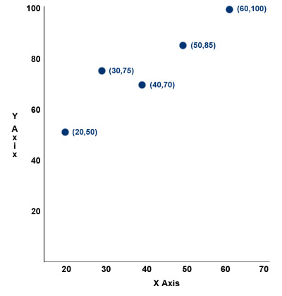
Axis example

You conduct a survey of typist test scores and find the following results: 100, 85, 70, 75, 50. Correspondingly, you find the age of each typist to be 60, 50, 40, 30, 20. What would be the x-axis if you were to plot this data?

Axis solution

The independent variable typically goes on the x-axis, in this case age, and the dependent variable, score, goes on the y-axis.

Example:

Age	Score
60	100
50	85
40	70
30	75
20	50

Slope and Intercept

An equation is most often expressed in the form:

y = mx + b

• m is the slope of a line in relation to the x-axis
• b is the intercept of the y-axis when x is equal to zero (x = 0)

The slope is the change in the value of y that corresponds directly to a change in the value of x.

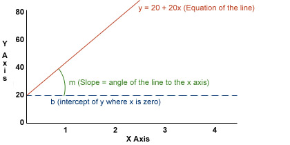
An equation is useful because it describes any value of y if you know any value of x.

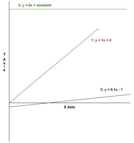
Slope and intercept example

Draw a graph that shows the following three lines:

1. The first line should show where the "x" value always equals the "y" value.
2. The second line should show where the "y" value is 10 less than the "x" value and an additional 10% more than the "x" value.
3. The third line should show the "y" value that is constant regardless of the value of "x."

Slope and intercept solution

The first line should show where the "x" value always equals the "y" value.	y = 1x + 0 y = x
The second line should show where the "y" value is 10 less than the "x" value and an additional 10% more than the "x" value.	y = (x - 10) 0.10 y = 0.1x - 1
The third line should show the "y" value that is constant regardless of the value of "x."	y = 0x + constant y = constant

Calculations of Equations

The equation of a straight line is:

y = mx + b

When given any two points on a line, one can calculate an equation to find any other points on the same line as follows:

Point 1 (x1y1)	Point 2 (x2y2)
Slope (m)
Intercept (b)	y1 - mx1
OR
Intercept (b)	y2 - mx2

Calculations of Equations Example

You have seen that a 60-year-old typist scored 100, while a 20-year-old typist scored 50 on a typing test. Calculate the equation for the line that passes through these points.

Calculations of Equations Solution

Point 1 (60,100)

Point 2 (20,50)

Slope (m)	50- 100 20 - 60 -50 - 40
Slope (m)	= 1.25
Intercept (b)	= y1 - mx1 = 100 - (1.25 x 60) = 100 - 75
Intercept (b)	= 25

The equation for the line that passes through (60,100) and (20,50) is:

y = 1.25x + 25

To check, review y₂ and x₂.

y₂ = mx₂ + b

50 = (1.25) (20) + 25

50 = 50

Correct

Footnotes